How to cite
If you find GRAND useful, please cite the following publication:Ben Guebila, Lopes-Ramos et al. GRAND: A database of gene regulatory network models across human conditions, NAR, 2022. doi:10.1093/nar/gkab778.
In addition, to cite a particular network model, the reference is available under the Reference section of each model.
Troubleshooting
- Supported browsers GRAND has been tested on Google Chrome (V92.0.4515.107), the Brave browser (V1.27.108), Firefox (V90.0.2), and Safari (V14.1.2). However, we do recommend Google Chrome for optimal user experience.
- Network graph does not display after clicking submit. GRAND uses thrid party libraries that are accessed remotly. Therefore, please make sure that browser security settings and firewall allow inbound channels.
- Network graph does not display in Brave browser Brave browser blocks GRAND by default and the security setting is set to 'shields up' by default. Set security settings to 'shields down' in the top right corner of the browser to allow network visualization.
- Exporting the network to png downloads a low resolution file The Save
as png button in network visualization allows to export the network as a png file. However the resolution depends on the screen resolution, therefore to get higher quality images, please increase your screen resolution.
1. Networks
A. Reconstruction
B. Download
Format:
Edg: stands for edges format. The network is written on a file with the following format:
                node1    node2    edge_weight

          e.g.,  A        B        1.0
or in the following format for multi-sample files:
                node1:node2    edge_weight_sample_1   edge_weight_sample_n

          e.g.,  A:B            1.0                    2.0
Adj: stands for Adjacency matrix format. The bipartite network is saved as the weighted adjacency matrix W(TFs,Genes).
gt: stands for gene targeting. Gene targeting is the sum of weighted in-degrees in the network.
tt: stands for TF targeting. TF targeting is the sum of weighted out-degrees in the network.
Networks are saved on 2 file extensions: First, a clear text
.csv or .txt file for most of the networks of GRAND. More recently, we started adopting binary .h5 files which use only 1/3 of memory space in comparison to clear text files.
Edge weights:
The edges weights are computed by PANDA, PUMA, OTTER, and LIONESS algorithms. They usually vary between -20 and 20. A large value means a high likelihood of the existence of an edge between two nodes, a low negative value means a small probability of interaction between two given nodes. For DRAGON, edges weights are partial correlations between the nodes.Download options are available in different formats. For example allows to download a network in
edges format with original edge weights.
2. Navigation
The following brief animated guide show to how to access a specific network and browse the phenotypic variables. Clicking the button in each page, takes you on step-by-step guide of the interface of the specific page or tool.Small molecule drugs

Cancer types

Tissues

Cell lines

Use case: drug repurposing in Melanoma
To illustrate specific use cases of GRAND, we will perform an integrated differential gene regulatory network analysis in Melanoma and predict small molecule drug that reverse this condition.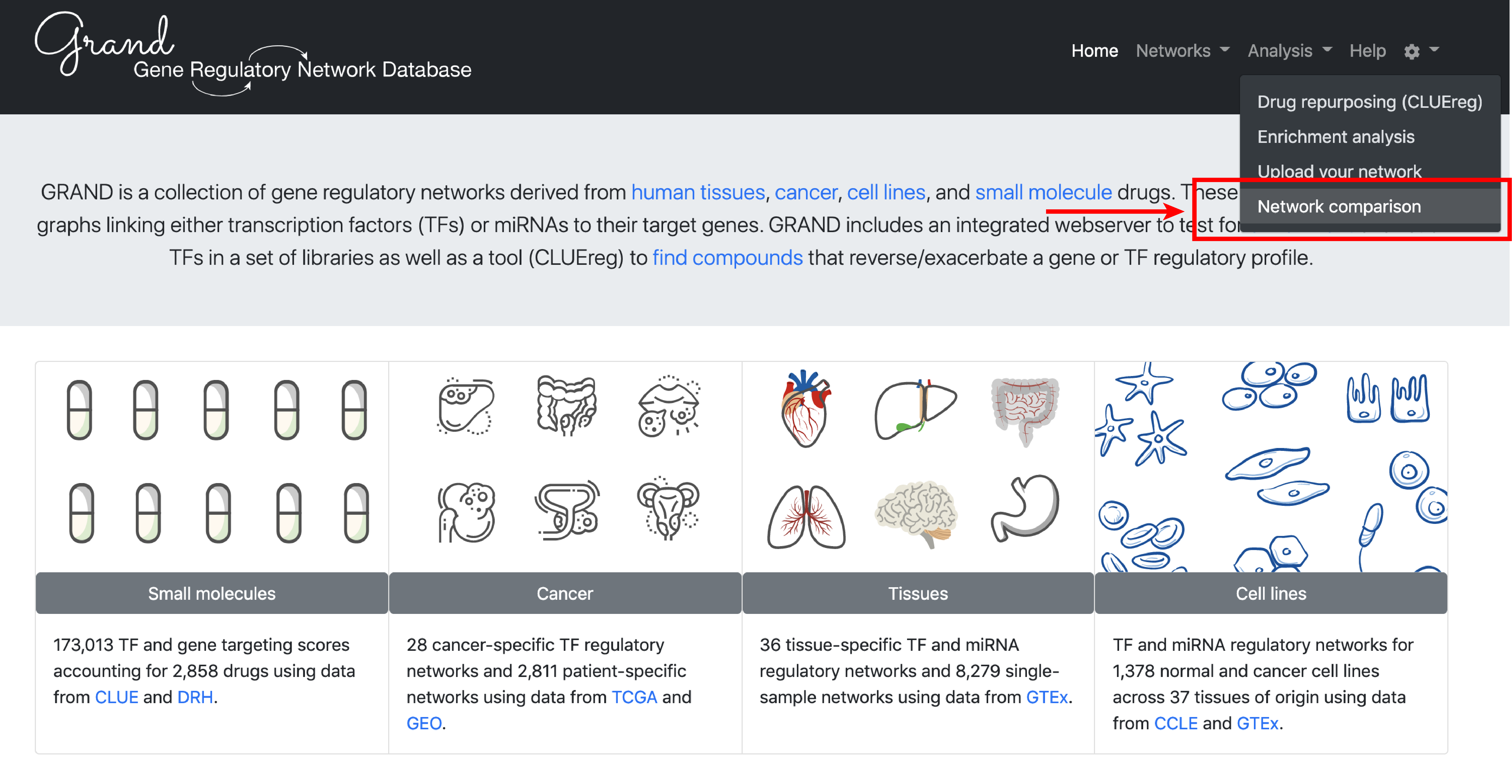
3. Analysis
The analysis section allows to analyse a set of TFs or genes in disease or small molecule category. It exploits the duality between TFs and genes in bipartite gene regulatory networks.
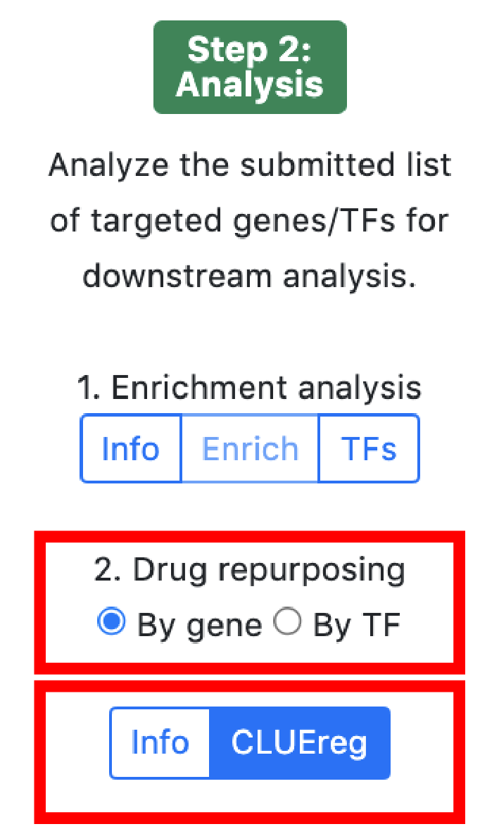
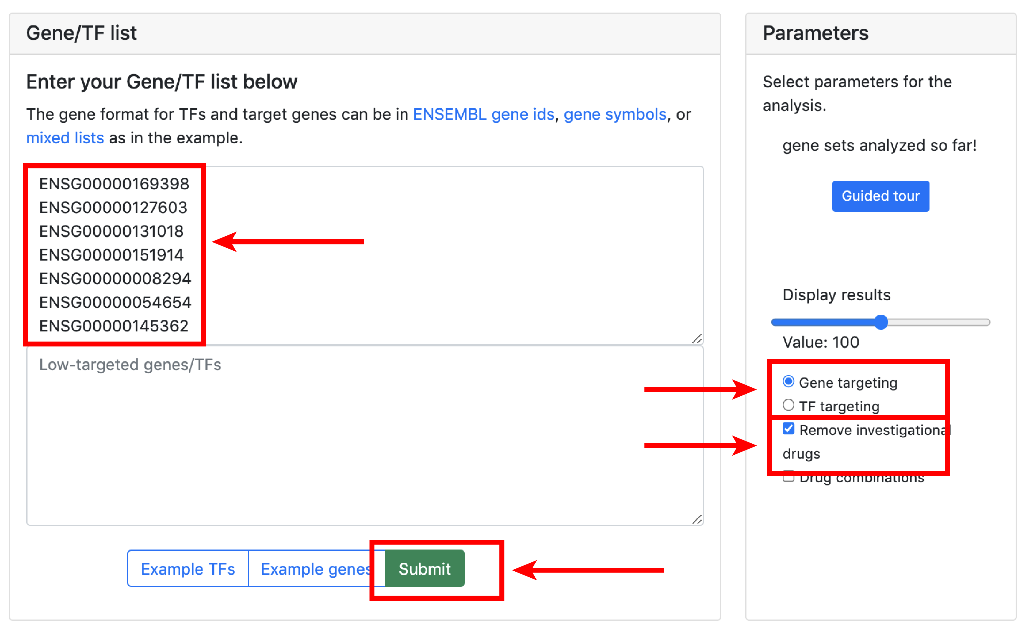
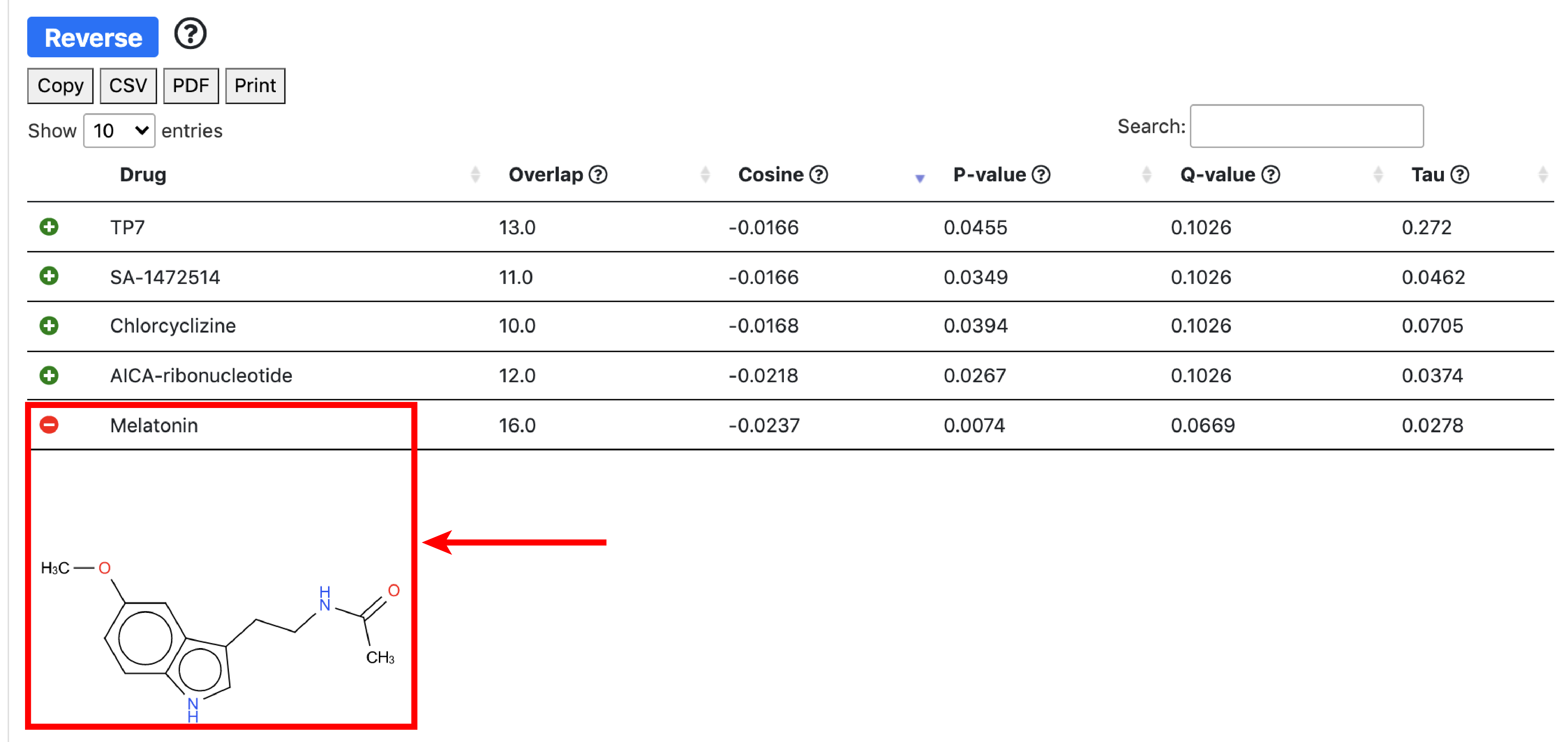
The small molecule analysis section allows to find compounds that optimally reverse the gene targeting or the transcription factor activity patterns in the query set.
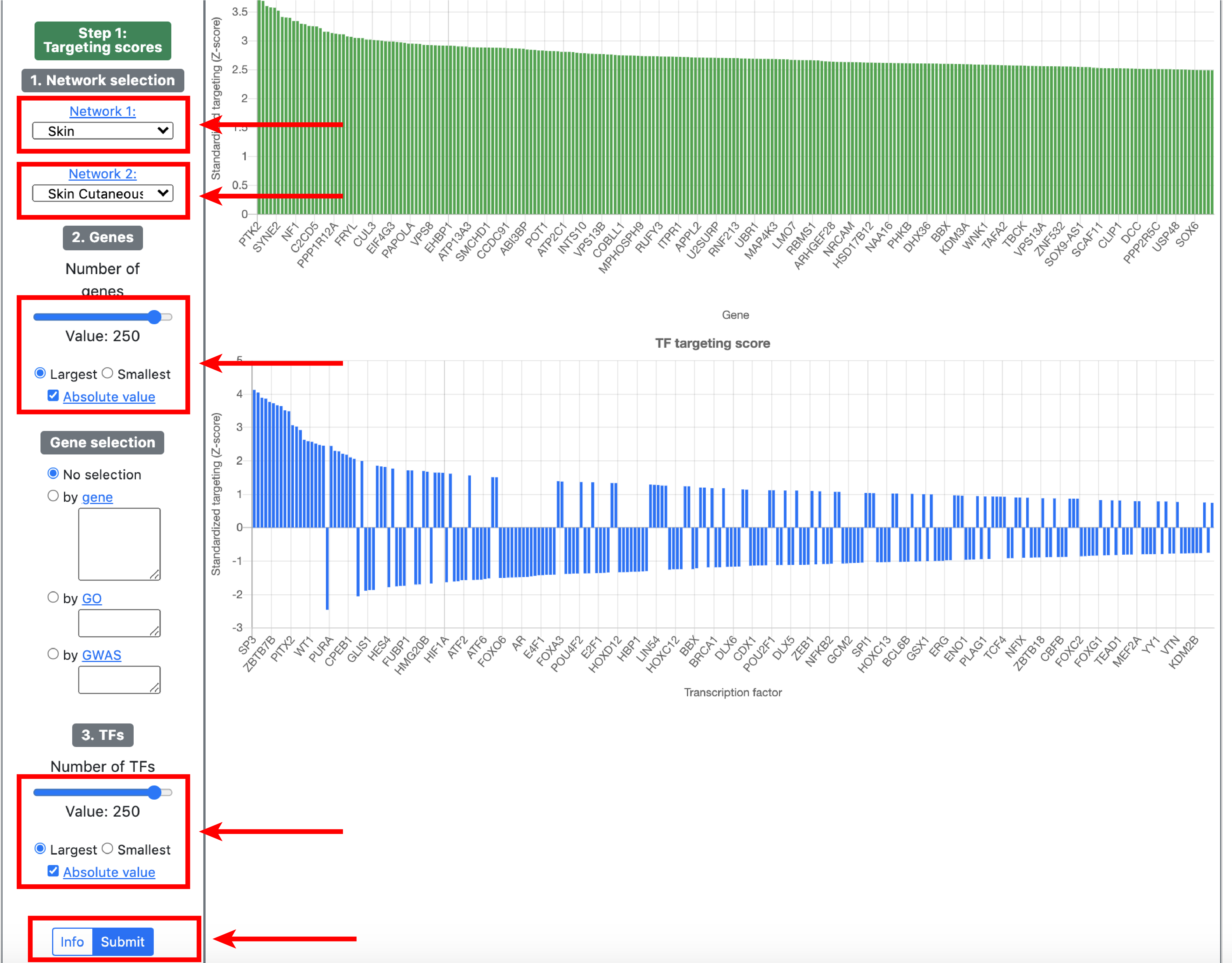
Gene targeting refers the to the weighted in-degree of a given gene. Since PANDA is usually validated against ChIP-seq data, targeting can be interpreted as the binding profile of TFs for a given gene in a particular experiment. Transcription targeting activity refers to the weighted out-degree of a given transcription factor. This tool serves for hypothesis generation wheras compounds that reverse/aggravate the gene/TF targeting patterns of a given experiment are hypothetical candidates for experimental validation.
The overlap score is equal to card(intersect(Input_Genes_Up,Drug_Genes_down)) + card(intersect(Input_Genes_Down,Drug_Genes_Up)) - card(intersect(Input_Genes_Up,Drugs_Genes_Up)) - card(intersect(Input_Genes_Down,Drugs_Genes_Down)). The cosine similarity compares the input vector to all the drugs. It is a signed measure that computes the direction of the vectors rather than their amplitude. In our case, we are interested in measuring the vectors of opposite directions, thus having negative cosine similarity.
4. Visualization
To enable network visualization, please make sure to use Google Chrome while navigating GRAND. The visualization module has 2 components. The first one allows to plot and query subgraphs of gene regulatory networks based on user selection. The second one allows to compute targeting scores from gene regulatory networks. Clicking the button on each page explains the parameters of the subnetwork selection and visualization.Network view

Targeting view

5. Wiki
PANDA
PANDA is a method that allows the inference of a TF to gene bipartite gene regulatory network by integrating three data sources: 1) gene coexpression, 2) TF PPI network, and 3) TF motif network. Details and examples can be found here. PANDA was compared to four other inference methods using ChIP-ChIP data in yeast in three conditions: TF knockout (KO), cell cycle (CC), and stress response (SR).OTTER
OTTER is an implementation of PANDA that uses convex optimization to infer the gene regulatory network. OTTER assumes that PPI and coexpression networks are projections of the regulatory network on the TF and Gene space and infers the network by optimzing graph matching between the three input networks. Details and examples can be found here. The accuracy of OTTER networks has been benchmarked against ChIP-seq data in breast cancer, liver cancer, and cervix cancer.PUMA
PUMA is an implementation of PANDA that infers miRNA to gene bipartite networks by integrating two data sources: 1) gene coexpression and 2) miRNA target networks. Details and examples can be found here.LIONESS
LIONESS allows to estimate single-sample gene regulatory networks from one aggregate network such as PANDA, PUMA, or coexpression networks. Details and examples can be found here.DRAGON
DRAGON allows the simultaneous inference of multi-layer Gaussian Graphical Model (GGM) omic networks. DRAGON allows the estimation of partial correlations using a low number of sample by implementing covariance shrinkage. Details and examples can be found here. DRAGON was compared to GGM for the accuracy to identify edges in single-cell multiomic dataset of simultaneously measured transcitptome and epitope (CITE-seq) for 6 diffrent sample sizes.EGRET
EGRET builds genotype-specific gene regualtory networks by integrating genomic variant information such as eQTLs and their effects on TF binding. EGRET seeds the PANDA algorithm with additional data that allows to reconstruct a network that is specific for a given genotype; these additional inputs are genotype data (vcf files), Qbic-pred prediction of TF biding alteration for each genotype, and eQTL data. Additional details and examples can be found here.Gene/TF/miRNA targeting
Targeting is a score for dircted bipartite networks. For source nodes (TFs/miRNA), targeting is the weighted outdegree, i.e., the sum of edge weights originating from the node. For target nodes (Genes), targeting is the weighted indegree, i.e., the sum of edge weights reaching the node. This score has been detailed in Weighill et al. 2021.GTEx
GTEx is a project that collected samples from 38 normal, non-disased tissues in humans and measured gene expression across each tissues. More details can be found here.TCGA
TCGA hosts gene expression data as well as other genomic information such as mutations, copy number variation and methylation for several cancer types in different tissues. More details can be found here.CCLE
CCLE datasets characterize more than 1500 human cell lines that model several cancer types across a large array of omic layers including copy number variation, mutations, methylation, protein and metabolite levels, alternative splicing, and chromatin marks quantification. More details can be found here.Connectivity Map
The connectivity map measured the activity of more than 20,000 approved and experimental small molecule compounds in normal and cancerous cell lines. The expression of 987 genes was measured using the L1000 assay and the expression of close to 11,000 genes were inferred from the 1000 genes set. More details can be found here.6. API
A. Documentation
B. Tutorial 1
    import requests
    import os
response=requests.get('https://grand.networkmedicine.org/api/v1/drugapi/')
responseFiltered=requests.get('https://grand.networkmedicine.org/api/v1/drugapi/?drug=1-phenylbiguanide')
To check that the data was collected correclty, we can do the following test.
    if response.status_code == 200:
    	print('Success!')
    elif response.status_code == 404:
    	print('Not Found.')
Since the API results are paginated for faster access, the previous command returns the first page with the first 50 drugs. To get the address of the next page, please use the following command:
data['next']
    data=response.json()
    drugs=data['results']
    for drug in drugs:
    	print(drug['drug'])
os.system('curl -O ' + drug['network'] + ' .')